Mathematics for Electrical Science and Physical Science 1. Module 1, linear systems, matrix rank, eigenvalues and diagonalization.

Module 1: Matrices and Linear Systems

Module outline

Linear systems of equations : Gauss elimination, Row echelon form, Linear Independence : rank of a matrix, Solutions of linear systems : Existence, Uniqueness (without proof), The matrix Eigen value Problem, Determining Eigen values and Eigen vector, Diagonalization of matrices.

Linear Systems of Equations.

A linear system of 'm' equations in 'n' unknowns $x_1, \dots, x_n$ is a set of equations of the form:

The system is called linear because each variable $x_j$ appears in the first power only.

• $a_{11}, \dots, a_{mn}$ are given numbers, called the coefficients of the system.

• $b_1, \dots, b_m$ on the right are also given numbers

Homogeneous Systems and Non-homogeneous System.

• If all the $b_j$ are zero, then the system is called a homogeneous system.
• If at least one $b_j$ is not zero, then the system is called a non homogeneous system.

Solutions of linear system.

• A solution of the system is a set of numbers $x_1, \dots, x_n$ that satisfies all the $m$ equations.
• If the system is homogeneous, it always has at least the trivial solution $x_1 = 0, \dots, x_n = 0$.
• When the system has at least one solution (one solution or infinitely many solutions) it is said to be consistent.
• When the system has no solution then the system is inconsistent system.

Matrix Form of the Linear system.

Matrix form of the Linear system: From the definition of matrix multiplication we see that the $m$ equations of the system may be written as a single vector equation.

$AX = B$

where the coefficient matrix $A = [a_{ij}]$ is a $m \times n$ matrix.

are column vectors.

we assume that the coefficients $a_{ij}$ are not all zero, so that $A$ is not a zero matrix.

Note that $x$ has $n$ components, whereas $B$ has $m$ components.

The matrix $\tilde{A} = \left[\begin{array}{ccc:c} a_{11} & \cdots & a_{1n} & b_1 \\ \vdots & & \vdots & \vdots \\ a_{m1} & \cdots & a_{mn} & b_m \end{array}\right]$ is called the augmented matrix of the system (1)

Note that the augmented matrix $\tilde{A}$ determines the system completely because it contains all the given numbers appearing in the system.

Geometric Interpretation, Existence and uniqueness of solutions.

If $m = n = 2$, we have two equations in two unknowns $x_1, x_2$

If we interpret $x_1, x_2$ as coordinates in the $x_1 - x_2$ - plane, then each of the two equations represents a straight line, and $(x_1, x_2)$ is a solution if and only if the point $P$ with coordinates $x_1, x_2$ lies on both lines. Hence there are three possible cases.

(a) Precisely one solution if the lines intersect (b) Infinitely many solutions if the lines coincide. (c) No solution if the lines are parallel.

Case (a)

Case (b)

Case (c)

Gauss Elimination and Back substitution

In the Gauss elimination method, the solution to the linear system of equations is obtained by.

Step 1 : First write the given system of equations into the matrix form.

$AX = B$

Step 2 : By elementary row operations, the augmented matrix $[AB]$ is brought to the upper triangular form.

Step 3 : The upper triangular system is solved using back substitution procedure by which we obtain the solution in the order $x_n, x_{n-1}, x_{n-2}, ext{...}, x_2, x_1$.

Example :

The Gauss elimination method can be motivated as follows. Consider a linear system that is in triangular form (in full, upper triangular form) such as

For instance, let the given system be,

Its augmented matrix is

We leave the first equation as it is. we eliminate $x_1$ from the second equation, to get a triangular system. For this we add twice the first equation to the second, and we do the same operation on the rows of the augmented matrix.

This gives $-4x_1 + 4x_1 + 3x_2 + 10x_2 = -30 + (2 \times 2)$,

that is,

$2x_1 + 5x_2 = 2$ $13x_2 = -26$

$\therefore x_1 = 6 \ , \ x_2 = -2$

Example :

Solve the system

$2x_1 + x_2 + 2x_3 + x_4 = 6$ $6x_1 - 6x_2 + 6x_3 + 12x_4 = 36$ $4x_1 + 3x_2 + 3x_3 - 3x_4 = -1$ $2x_1 + 2x_2 - x_3 + x_4 = 10$

Step 1 : The given system of equations can be brought to the form.

$AX = B$

by writing it as

Step 2 : Now the augmented matrix $[AB]$ is brought to the upper triangular form as below:

Hence the corresponding matrix equation is,

\begin{bmatrix} 2 & 1 & 2 & 1 \ 0 & -9 & 0 & 9 \ 0 & 0 & -1 & -4 \ 0 & 0 & 0 & 13 \end{bmatrix} \begin{bmatrix} x_1 \ x_2 \ x_3 \ x_4 \end{bmatrix}

\begin{bmatrix} 6 \ 18 \ -11 \ 39 \end{bmatrix}

\begin{aligned} 2x_1 + x_2 + 2x_3 + x_4 &= 6 & \cdots\cdots (1) \ -9x_2 + 9x_4 &= 18 & \cdots\cdots (2) \ -x_3 - 4x_4 &= -11 & \cdots\cdots (3) \ 13x_4 &= 39 & \cdots\cdots (4). \end{aligned}

Step 3 : [Back substitution]

From (4), we obtain $x_4 = 3$.

Substituting this value in (3), we obtain $x_3 = -1$.

Using these values, (2) gives $x_2 = 1$.

Putting all these values in (1), we obtain $x_1 = 2$.

Hence the solution to the given system of equations is $x_1 = 2, x_2 = 1, x_3 = -1, x_4 = 3$

Example :

Solve the linear system.

$x_1 - x_2 + x_3 = 0 \quad \text{--- } (1)$ $30x_2 - 20x_3 = 80 \quad \text{--- } (2)$ $95x_3 = 190 \quad \text{--- } (3)$

$\therefore x_3 = 2$

substitute in $(2)$ $\Rightarrow 30x_2 - 40 = 80$ $30x_2 = 120$ $\therefore x_2 = 4$

substitute in $(1)$ $\Rightarrow x_1 - x_2 + x_3 = 0$ $x_1 = x_2 - x_3$ $x_1 = 4 - 2$ $\underline{\therefore x_1 = 2}$

Elementary Row Operations.

Elementary Row Operations for Matrices:

Interchange of two rows

Addition of a constant multiple of one row to another row.

Multiplication of a row by a non zero constant 'c'

Elementary operations for Equations.

• Interchange of two equations
• Addition of a constant multiple of one equation to another equation
• Multiplication of an equation by a non zero constant '$c$'.

Row - Equivalent systems :

We now call a linear system $S_1$ row-equivalent to a linear system $S_2$ if $S_1$ can be obtained from $S_2$ by (finitely many!) row operations. This justifies Gauss elimination and establishes the following result.

Theorem.

• Systems having the same solution sets are often called $\underline{\text{equivalent systems}}$.

Gauss Elimination : The Three Possible cases of systems.

1.) Gauss elimination if unique solution exists

2.) Gauss elimination if infinitely many solutions exist.

3.) Gauss elimination if no solution exists.

Gauss Elimination if infinitely Many solutions exist

solve the following linear system of three equations in four unknowns whose augmented matrix is:

Thus,

Solution: As in the previous example, we circle pivots and box terms of equations and corresponding entries to be eliminated. We indicate the operations in terms of equations and operate on both equations and matrices.

Step 1. Elimination of $x_1$ from the second and third equations by adding

$-0.6 / 3.0 = -0.2 \text{ times the first equation to the second equation,}$

$-1.2 / 3.0 = -0.4 \text{ times the first equation to the third equation.}$

This gives the following, in which the pivot of the next step is circled.

$3.0 x_1 + 2.0 x_2 + 2.0 x_3 - 5.0 x_4 = 8.0$ $(1.1 x_2) + 1.1 x_3 - 4.4 x_4 = 1.1$ $[-1.1 x_2] - 1.1 x_3 + 4.4 x_4 = -1.1$

Step 2. Elimination of $x_2$ from the third equation by adding $1.1 / 1.1 = 1$ times the second equation to the third equation.

This gives,

since $x_3$ and $x_4$ remain arbitrary, we have infinitely many solutions. If we choose a value of $x_3$ and a value of $x_4$, then the corresponding values of $x_1$ and $x_2$ are uniquely determined.

Gauss Elimination if no solution Exists.

Consider

Step 1. Elimination of $x_1$ from the second and third equations by adding.

$-\frac{2}{3}$ times the first equation to the second equation,

$-\frac{6}{3} = -2$ times the first equation to the third equation.

This gives

Step 2. Elimination of $x_2$ from the third equation gives

The false statement $0 = 12$ shows that the system has no solution.

Row Echelon form.

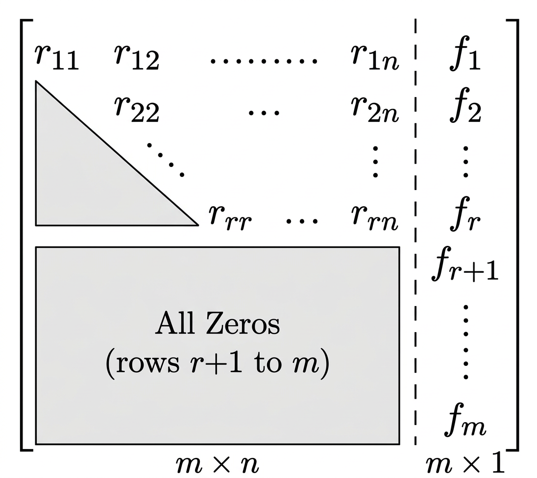
At the end of the Gauss elimination the form of the coefficient matrix, the augmented matrix, and the system itself are called the row echelon form. In it, rows of zeros, if present, are the last rows, and, in each non zero row, the leftmost non zero entry is farther to the right than in the previous row.

The original system of '$m$' equations in '$n$' unknowns has augmented matrix $[A|B]$. This is to be row reduced to matrix $[R|F]$. The two systems $AX = B$ and $RX = F$ are equivalent:

if either one has a solution, so does the other, and the solutions are identical.

At the end of the Gauss elimination (before the back substitution), the row echelon form of the augmented matrix will be,

Here, $r \le m$, $r_{11} \ne 0$, and all entries in the blue triangle and blue rectangle are zero.

The Rank.

The rank of a matrix in Row-Echelon form is equal to the number of non-zero rows.

The rank of a matrix is also given by the number of linearly independent rows.

$\text{If } A \text{ is zero matrix, then } r(A) = 0$ $\text{If } A \text{ is not a zero matrix, } r(A) \ge 1$

Note:

(a) No solution: If $r$ is less than $m$ (meaning that $R$ actually has at least one row of all $0$s) and at least one of the numbers $f_{r+1}, f_{r+2}, \dots, f_m$ is not zero, then the system $RX = F$ is inconsistent: No solution is possible. Therefore the system $AX = B$ is inconsistent as well.

(b) Unique solution. If the system is consistent and $r = n$ there is exactly one solution, which can be found by back substitution.

(c) Infinitely many solutions. To obtain any of these solutions, choose values of $x_{r+1}, \dots, x_n$ arbitrarily. Then solve the $r^{\text{th}}$ equation for $x_r$ (in terms of those arbitrary values), then the $(r-1)^{\text{st}}$ equation for $x_{r-1}$ and so on up the line.

Linear Independence and Dependence of vectors.

Given any set of $m$ vectors $a_{(1)}, \dots, a_{(m)}$ (with the same number of components), a linear combination of these vectors is an expression of the form.

$\boxed{c_1 a_{(1)} + c_2 a_{(2)} + \dots + c_m a_{(m)}}$

where $c_1, c_2, \dots, c_m$ are any scalars. Now consider the equation.

$c_1 a_{(1)} + c_2 a_{(2)} + \dots + c_m a_{(m)} = 0$

clearly, this vector equation holds if we choose all $c_j$'s zero, because then it becomes $0 = 0$. If this is the only $m$-tuple of scalars for which it holds, then our vectors $a_{(1)}, \dots, a_{(m)}$ are said to form a linearly independent set or, more briefly, we call them linearly independent. Otherwise, if it also holds with scalars not all zero, we call these vectors linearly dependent.

This means that we can express at least one of the vectors as a linear combination of the other vectors. For instance, if (1) holds with, say, $c_1 \neq 0$, we can solve it for $a_{(1)}$:

$a_{(1)} = k_2 a_{(2)} + \dots + k_m a_{(m)} \quad \text{where } k_j = -c_j / c_1$

(some $k_j$'s may be zero. Or even all of them, namely, if $a_{(1)} = 0$.)

Remark: Any set of $m$ vectors $a_{(1)}, \dots, a_{(m)}$ is linearly independent if $c_1 a_{(1)} + c_2 a_{(2)} + \dots + c_m a_{(m)} = 0$ implies $c_1 = c_2 = \dots = c_m = 0$.

Example: Examine the linear independence of the three vectors.

Solution:

The given three vectors are linearly dependent because $a_{(1)} + a_{(2)} - a_{(3)} = [0 \quad 0 \quad 0] = 0$

The first two of the three vectors are linearly independent : because $c_1 a_{(1)} + c_1 a_{(2)} = [0 \quad 0 \quad 0] = 0$

implies $[c_1 + 2c_2 \quad 2c_1 + 3c_2 \quad 3c_1 + 4c_2] = [0, 0 \quad 0]$

implies $c_1 + 2c_2 = 0, \quad 2c_1 + 3c_2 = 0, \quad \text{and} \quad 3c_1 + 4c_2 = 0$

The first one of these equations gives $c_1 = -2c_2$ which substituting on the second equation yields $c_2 = 0$ which implies $c_1 = -2c_2 = -2 \times 0 = 0$.

Hence $c_1 = 0$ and $c_2 = 0$.

Example: find whether the vectors $[1 \quad 2 \quad -1 \quad 3], [2 \quad -1 \quad 3 \quad 2], [-1 \quad 8 \quad -9 \quad 3]$ are linearly independent.

solution $c_1 [1 \quad 2 \quad -1 \quad 3] + c_2 [2 \quad -1 \quad 3 \quad 2] + c_3 [-1 \quad 8 \quad -9 \quad 3] = [0 \quad 0 \quad 0 \quad 0]$

implies

Hence we have the system of equations:

$c_1 + 2c_2 - c_3 = 0$ $-5c_2 + 10c_3 = 0$ $-2c_3 = 0$

gives by back substitution

$c_3 = 0, \quad c_2 = 0, \quad c_1 = 0$

Hence the given set of vectors is linearly independent.

Rank of a matrix

The rank of a matrix $A$ is the maximum number of linearly independent row vectors of $A$. It is denoted by $\text{rank } A$.

The matrix

first two row vectors are linearly independent,

whereas all three row vectors are linearly dependent.

We call a matrix $A_1$ row-equivalent to a matrix $A_2$ if $A_1$ can be obtained from $A_2$ by (finitely many!) elementary row operations.

Now the maximum number of linearly independent row vectors of a matrix does not change if we change the order of rows or multiply a row by a nonzero $c$ or take a linear combination by adding a multiple of a row to another row. This shows that rank is invariant under elementary row operations:

THEOREM 1

Row-Equivalent Matrices.
Row-equivalent matrices have the same rank.

Once the matrix is in row-echelon form, we count the number of nonzero rows, which is precisely the rank of the matrix.

Determination of Rank.

The last matrix is in row-echelon form and has two non zero rows. Hence $\operatorname{rank} A = 2$, as before.

THEOREM 2

Linear Independence and Dependence of vectors.

Consider $p$ vectors that each have $n$ components. Then these vectors are linearly independent if the matrix formed, with these vectors as row vectors, has rank $p$. However, these vectors are linearly dependent if that matrix has rank less than $p$.

THEOREM 3

Rank in Terms of Column vectors

The rank $r$ of a matrix $A$ equals the maximum number of linearly independent column vectors of $A$.

Hence $A$ and its transpose $A^T$ have the same rank.

VECTOR SPACE

A vector space is a (non empty) set $V$ of vectors with the same number of components such that with any two vectors $a$ and $b$ in $V$ all their linear combinations $\alpha a + \beta b$ ($\alpha, \beta$ any real numbers) are elements of $V$, and these vectors satisfy the following laws:

• A1 : $a + b = b + a$
• A2 : $(a + b) + c = a + (b + c)$ (written $a + b + c$)
• A3 : $a + 0 = a$
• A4 : $a + (-a) = 0$.

$M1 : \alpha (a+b) = \alpha a + \alpha b$
$M2 : (\alpha + \beta) a = \alpha a + \beta a$
$M3 : \alpha (\beta a) = (\alpha \beta) a$ (written $\alpha \beta a$)
$M4 : 1a = a$

The maximum number of linearly independent vectors in $V$ is called the dimension of $V$ and is denoted by $\dim V$.

A linearly independent set in $V$ consisting of a maximum possible number of vectors in $V$ is called a basis for $V$. In other words, any largest possible set of independent vectors in $V$ forms basis for $V$. That means, if we add one or more vector to that set, the set will be linearly independent.

THEOREM 6

Row space and Column space
The row space and the column space of a matrix $A$ have the same dimension, equal to $\text{rank } A$.

Example: Find the rank and a basis for the row space and for the column space of the matrix.

The last matrix is in row echelon form and since it has only one non zero row, rank of that matrix and hence that of the given matrix is 1.

Also, a basis for the row space of $A$ is $\begin{bmatrix} 1 & -2 \end{bmatrix}$

To find a basis for the column space, we find the row echelon form of $A^T$.

Hence a basis for the row space of $A^T$ is $\begin{bmatrix} 1 & 0 & -3 \end{bmatrix}$

Hence a basis for the column space of $A$ is $\begin{bmatrix} 1 \\ 0 \\ -3 \end{bmatrix}$

Solutions of Linear Systems: Existence, Uniqueness.

A linear system in $n$ unknowns has a unique solution if the coefficient matrix and the augmented matrix have the same rank $n$, and infinitely many solutions if that common rank is less than $n$. The system has no solution if those two matrices have different rank.

Fundamental theorem for Linear Systems.

(a) Existence. A linear system of $m$ equations

$x_1, \dots, x_n$ :

is consistent, that is, has solutions, if and only if the coefficient matrix $A$ and the augmented matrix $\tilde{A}$ have the same rank. Here,

and $\tilde{A} = \left[\begin{array}{ccc:c} a_{11} & \cdots & a_{1n} & b_1 \\ \vdots & \cdots & \vdots & \vdots \\ a_{m1} & \cdots & a_{mn} & b_m \end{array}\right]$

(b) Uniqueness. The system has precisely one solution if and only if this common rank $r$ of $A$ and $\tilde{A}$ equals $n$.

(c) Infinitely many solutions. If this common rank $r$ is less than $n$, the system has infinitely many solutions. All of these solutions are obtained by determining $r$ suitable unknowns (whose submatrix of coefficients must have rank $r$.) in terms of the remaining $n-r$ unknowns, to which arbitrary values can be assigned.

d.) Gauss elimination : If solution exist, they can all be obtained by the Gauss elimination. This method will automatically reveal whether or not solutions exist.

Homogeneous Linear system.

A homogeneous linear system.

always has the trivial solution $x_1 = 0, \dots, x_n = 0$. Non trivial solutions exist if and only if $\text{rank } A < n$. If $\text{rank } A = r < n$, these solutions, together with $x=0$, form a vector space of dimension $n-r$, called the solution space.

In particular, if $x_{(1)}$ and $x_{(2)}$ are solution vectors, then $x = c_1 x_{(1)} + c_2 x_{(2)}$ with any scalars $c_1$ and $c_2$ is a solution vector. (This does not hold for nonhomogeneous systems. Also, the term solution space is used for homogeneous systems only.)

• Test for consistency and solve the system of equations.

  $x + 2y - z = 3 \quad , \quad 3x - y + 2z = 1$ $2x - 2y + 3z = 2 \quad , \quad x - y + z = -1$

  $AX = B$

  $$$$

[AB] = \left[\begin{array}{ccc:c} 1 & 2 & -1 & 3 \ 3 & -1 & 2 & 1 \ 2 & -2 & 3 & 2 \ 1 & -1 & 1 & -1 \end{array}\right]

Matrix Eigenvalue Problems.

A matrix eigen value problem considers the vector equation.

$\boxed{Ax = \lambda x}$

Here $A$ is a given square matrix, $\lambda$ an unknown scalar, and $x$ an unknown vector. In a matrix eigen value problem, the task is to determine $\lambda$'s and $x$'s that satisfy. Since $x = 0$ is always a solution for any $\lambda$ and thus not interesting, we only admit solutions with $x \neq 0$.

The solutions are given the following names: The $\lambda$'s that satisfy are called eigenvalues of $A$ and the corresponding non zero $x$'s that also satisfy are called eigenvectors of $A$.

Consider multiplying non zero vectors by a given square matrix, such as,

we introduce more terminology. A value of $\lambda$, for which it has a solution $x \neq 0$, is called an eigen value or characteristic value of the matrix $A$. Another term for $\lambda$ is a latent root. ("Eigen" is German and means "proper" or "characteristic".)

The corresponding solutions $x \neq 0$ are called the eigen vectors or characteristic vectors of $A$ corresponding to that eigen value $\lambda$. The set of all the eigenvalues of $A$ is called the spectrum of $A$.

we shall see that the spectrum consists of atleast one eigenvalue and at most of $n$ numerically different eigenvalues. The largest of the absolute values of the eigen values of $A$ is called the spectral radius of $A$.

How to find Eigen values and Eigenvectors ?

• We illustrate all the steps in terms of the matrix $A = \begin{bmatrix} -5 & 2 \\ 2 & -2 \end{bmatrix}$

$Ax = \lambda x$

$-5x_1 + 2x_2 = \lambda x_1$ $2x_1 - 2x_2 = \lambda x_2$

$-5x_1 + 2x_2 - \lambda x_1 = 0$ $(-5 - \lambda)x_1 + 2x_2 = 0$ $(-2 - \lambda)x_2 + 2x_1 = 0$

$\lambda^2 + 7\lambda + 6 = 0$ $(\lambda + 1)(\lambda + 6) = 0$ $\therefore \lambda = -1, -6$

when $\lambda = -1$

\begin{bmatrix} -4 & 2 \ 2 & -1 \end{bmatrix} \begin{bmatrix} x_1 \ x_2 \end{bmatrix} = 0$$

$-4x_1 + 2x_2 = 0$ $2x_1 - x_2 = 0$

$\Rightarrow -2x_1 + x_2 = 0$

Put, $x_1 = a$ $x_2 = 2a$

$a = 1$

when $\lambda = -6$

\begin{bmatrix} 1 & 2 \ 2 & 4 \end{bmatrix} \begin{bmatrix} x_1 \ x_2 \end{bmatrix} = 0$$

$x_1 + 2x_2 = 0$ $2x_1 + 4x_2 = 0$

$\Rightarrow 3x_1 + 6x_2 = 0$ $x_1 + 2x_2 = 0$

Put $x_1 = a$ $x_2 = -\frac{a}{2}$

$a = 2$

This example illustrates the general case as follows. Equation written in components is

$a_{11}x_1 + \dots + a_{1n}x_n = \lambda x_1,$ $a_{21}x_1 + \dots + a_{2n}x_n = \lambda x_2$

$- - - - - - - - - - - - - - - - - - - - -$

$a_{n1}x_1 + \dots + a_{nn}x_n = \lambda x_n$

Transferring the terms on the right side to the left side, we have,

In matrix notation, $\boxed{(A - \lambda I) x = 0}$

By Cramer's theorem, this homogeneous linear system of equations has a non trivial solution if and only if the corresponding determinant of the coefficients is zero:

$\boxed{\lambda^2 - (\operatorname{tr} A)\lambda + |A| = 0}$ characteristic equation.

$\lambda^2 - 16\lambda + 48 = 0$ $\Rightarrow \lambda = 4, 12$

For $\lambda = 4$

$[A - 4I]x = 0$

$6x_1 + 3x_2 = 0$ $4x_1 + 2x_2 = 0$

on solving, $2x_1 + x_2 = 0$ $\text{Let, } x_1 = k, \ x_2 = -2k$

for $\lambda = 12$

$[A - 12I]x = 0$

\begin{bmatrix} -2 & 3 \ 4 & -6 \end{bmatrix} \begin{bmatrix} x_1 \ x_2 \end{bmatrix} = 0$$-2x_1 + 3x_2 = 0$$4x_1 - 6x_2 = 0$$

on solving $2x_1 - 3x_2 = 0$ $\text{put } x_1 = k, \ x_2 = \frac{2}{3}k$

for $k = 1$, $\begin{bmatrix} x_1 \\ x_2 \end{bmatrix} = \begin{bmatrix} 1 \\ \frac{2}{3} \end{bmatrix}$

$k = 3$, $\begin{bmatrix} x_1 \\ x_2 \end{bmatrix} = \begin{bmatrix} 3 \\ 2 \end{bmatrix}$

Q:- Find eigen values and eigen vectors of the matrix $A = \begin{bmatrix} 8 & -4 \\ 2 & 2 \end{bmatrix}$

$\lambda^2 - (\text{tr} A)\lambda + |A| = 0$

$|A - \lambda I| = 0$

\begin{bmatrix} 8 - 4 & -4 \ 2 & 2 - 4 \end{bmatrix} \begin{bmatrix} x \ y \end{bmatrix} = \begin{bmatrix} 0 \ 0 \end{bmatrix}

\begin{bmatrix} 4 & -4 \ 2 & -2 \end{bmatrix} \begin{bmatrix} x \ y \end{bmatrix} = \begin{bmatrix} 0 \ 0 \end{bmatrix}

\begin{bmatrix} x \ y \end{bmatrix} = \begin{bmatrix} k \ k \end{bmatrix} = k \begin{bmatrix} 1 \ 1 \end{bmatrix}

$\underline{\lambda = 6}$

$[A - 6I]X = 0$

$2x - 4y = 0$ $\Rightarrow x - 2y = 0$

Let, $x = k$, $y = \frac{k}{2}$